Solving Linear Equations
Lecture 6
Recap
$$ % Colors
% Coordinate vectors and matrices
% Common sets
% Abstract vector symbols
% Norms / absolute value
% Optional: dot product spacing (looks nicer in slides)
% Operators $$
Linear transformations
- A linear transformation \(A:\mathbb{R}^k \to \mathbb{R}^n\) maps a vector \(\vec{x}\in\mathbb{R}^k\) to \(A\vec{x}\in\mathbb{R}^n\) via multiplication by an \(n\times k\) matrix \(A\).
- The transformation is completely determined by its action on the coordinate vectors \(\vec{e}_i\in\mathbb{R}^k\), sending each to a vector \(\vec{v}_i\in\mathbb{R}^n\).
- Each vector \(\vec{v}_i=A\vec{e}_i\) appears as the \(i\)-th column of \(A\). Equivalently, knowing \(A\vec{e}_i\) for all \(i\) determines the matrix.
- In low dimensions—especially in the plane—these effects can often be visualized geometrically.
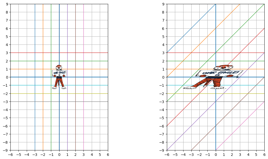
Example: \(A(x,y)=(3x+y,\,y)\)
- What are \(A\vec{e}_1\) and \(A\vec{e}_2\)? They are exactly the column vectors of \(A\).
Solving linear equations
Motivation
- A function \(f(x)=y\) describes the relationship between an input (\(x\)) and an output (\(y\)).
- In practice, we often want to determine the input given an observed or measured output.
- Example: “I spent $50 this month at coffee shops. How much coffee did I drink and how many bagels did I have? How should I adjust my habits to spend only $30 a month?”
Linear equations
- Linear maps (transformations) are fundamental because many functions can be well approximated by linear ones, and linear problems are much easier to solve.
- Fact: if a function is differentiable, then it can be approximated by a linear function; this also holds in higher dimensions (see multivariable calculus).
- Therefore, solving equations of the form \[A\vec{x}=\vec{b}\] for a given \(\vec{b}\) is very important.
- Such an equation is called a linear equation.
Notational convention
- Let \(\vec{x}=\langle x_1,\dots,x_m \rangle\) be the vector of \(m\) unknown variables.
- Let \[A=\begin{bmatrix} a_{11}&\cdots&a_{1m}\\ \vdots&\ddots&\vdots\\ a_{n1}&\cdots&a_{nm} \end{bmatrix}\] be an \(n\times m\) coefficient matrix.
- Let \(\vec{b}=\langle b_1,\dots,b_n \rangle\) be a given vector.
- Our goal is to solve \(A\vec{x}=\vec{b}\) for the unknowns \(x_1,\dots,x_m\).
System of linear equations
- Writing the equation coordinate by coordinate gives the system of linear equations \[\left\{\begin{aligned} a_{11}x_1+\cdots+a_{1m}x_m &= b_1\\ &\vdots\\ a_{n1}x_1+\cdots+a_{nm}x_m &= b_n. \end{aligned}\right.\]
- You are probably already familiar with solving equations of this form!
Gaussian elimination
- Gaussian elimination is a systematic algorithm for solving systems of linear equations.
- The idea is to eliminate variables step by step using existing equations.
- In the end, the system may have a unique solution, infinitely many solutions, or no solution.
Elementary row operations
- Interchange two equations.
Notation: \(R_i\leftrightarrow R_j\) - Multiply an equation by a nonzero constant.
Notation: \(R_i\leftarrow cR_i\), \(c\neq0\) - Add a multiple of one equation to another.
Notation: \(R_i\leftarrow R_i+cR_j\)
Steps for Gaussian elimination
- Ensure the first equation has a nonzero coefficient of \(x_1\) (swap equations if necessary).
- Scale this equation to obtain a convenient leading coefficient.
- Subtract suitable multiples of this equation from the others to eliminate \(x_1\).
- Repeat for the remaining variables \(x_2,\dots,x_m\).
Augmented matrix
- To keep track of these steps efficiently, we record only the coefficients and constants.
- The \(n\times(m+1)\) matrix \[[A\mid\vec{b}] = \left[\begin{array}{ccc|c} a_{11}&\cdots&a_{1m}&b_1\\ \vdots&\ddots&\vdots&\vdots\\ a_{n1}&\cdots&a_{nm}&b_n \end{array}\right]\] is called the augmented matrix.
Example
- Solve the system of linear equations \[\left\{\begin{aligned} x+y+z &= 6\\ 2x-y+z &= 3\\ -x+2y+z &= 6 \end{aligned}\right.\]
Gaussian elimination
- Eliminate \(x\) from the second and third rows: \[\left[\begin{array}{ccc|c} 1&1&1&6\\ 2&-1&1&3\\ -1&2&1&6 \end{array}\right]\\ \xrightarrow{\substack{R_2\leftarrow R_2-2R_1\\[2pt] R_3\leftarrow R_3+R_1}} \left[\begin{array}{ccc|c} 1&1&1&6\\ 0&-3&-1&-9\\ 0&3&2&12 \end{array}\right].\]
Continue elimination
- Eliminate \(y\) from the third row: \[\xrightarrow{R_3\leftarrow R_3+R_2} \left[\begin{array}{ccc|c} 1&1&1&6\\ 0&-3&-1&-9\\ 0&0&1&3 \end{array}\right].\]
Back substitution
- Solve from the bottom up: \[\begin{align*} &z=3,\\ -3y-z=-9\ \Rightarrow\ &y=2,\\ x+y+z=6\ \Rightarrow\ &x=1.\end{align*}\]
- This is called the back substitution.
Gauss–Jordan elimination
- By incorporating back substitution into elimination, we can simplify the augmented matrix further.
- Eliminate variables above each leading entry (the first nonzero entry of each row).
- Scale each row so the leading coefficient is \(1\).
- This procedure is called Gauss–Jordan elimination.
Reduced row-echelon form
- The final matrix obtained after Gauss–Jordan elimination is in reduced row-echelon form (RREF).
- Each leading entry is \(1\) and is the only nonzero entry in its column.
- Any rows consisting entirely of zeros for coefficients (if present) appear at the bottom.
RREF (Case 1: unique solution)
\[ \left[\begin{array}{ccc|c} 1 & 0 & 0 & 2\\ 0 & 1 & 0 & -1\\ 0 & 0 & 1 & 3 \end{array}\right] \]
- Every row has a leading entry (also called a pivot).
- Each variable is uniquely determined by the augmented values.
- The number of equations matches the number of variables, so the system is neither overdetermined nor underdetermined.
RREF (Case 2: infinitely many solutions)
\[ \left[\begin{array}{cccc|c} 1 & 0 & 3 & 0 & 2\\ 0 & 0 & 0 & 1 & -1\\ 0 & 0 & 0 & 0 & 0 \end{array}\right] \quad\text{or}\quad \left[\begin{array}{cccc|c} 1 & 0 & -1 & 2 & 4\\ 0 & 1 & 3 & -1 & -2 \end{array}\right] \]
- The number of leading entries (nonzero rows) is less than the number of variables.
- Any variable without a leading entry is a free variable and may take arbitrary values.
- All other variables are uniquely determined in terms of the free variables.
- Free variables are also called parameters.
RREF (Case 3: possibly no solution)
\[ \left[\begin{array}{ccc|c} 1 & 0 & 2 & 3\\ 0 & 1 & -1 & 4\\ 0 & 0 & 0 & c \end{array}\right] \]
- Some bottom rows have no leading entry in their coefficient part.
- If \(c\neq0\), such a row represents the equation \(0=c\), so the system is inconsistent and has no solution.
- If \(c=0\), the row represents the identity \(0=0\) and can be ignored.
- After removing all zero rows, the system falls into either the unique-solution case or the infinitely-many-solutions case.
Summary
- A linear equation has the form \(A\vec{x}=\vec{b}\), where \(A\) is an \(n\times m\) matrix, \(\vec{x}\in\mathbb{R}^m\) is the vector of unknowns, and \(\vec{b}\in\mathbb{R}^n\) is the given vector.
- The terms linear equation and system of linear equations are often used interchangeably.
- The corresponding augmented matrix is written as \([A\mid\vec{b}]\).
- To solve a system of linear equations, we apply Gauss–Jordan elimination to the augmented matrix using elementary row operations to obtain the reduced row-echelon form (RREF).
- Depending on the final RREF, the system may have a unique solution, infinitely many solutions, or no solution.
Comments